5. MCMC in practice#
Last week we have seen that Markov Chain Monte Carlo simulations work in theory. We can summarize our findings as follows. Given a discrete or continuous state space \(\Gamma\), a desired probability distribution \(\pi\) on \(\Gamma\), and an observable \(f:\Gamma \to \mathbb{R}\), the problem is to compute the expectation value of \(f\) evaluated on a random variable \(X\) on \(\Gamma\) with probability mass function or probability density functions given by \(\pi\),
In the discrete case this problem can be addressed by designing a Markov chain transition matrix \(P(x\to y)\) that is irreducible and has \(\pi\) as its stationary distribution, i.e. \(\pi P = \pi\). One then considers the Markov chain \(X_0,X_1,X_2,\ldots\) with arbitrary distribution for \(X_0\) and transition probability dictated by \(P(x\to y)\). The ergodic theorem then assures us that we can approximate \(\mathbb{E}[f(X)]\) via the time average
The same holds in the continuous case for an irreducible transition density, under a technical additional assumption of Harris recurrence.
We have also seen how to obtain a suitable transition matrix \(P(x\to y)\) from a proposal transition matrix \(Q(x\to y)\) using the Metropolis-Hastings algorithm. Thus with infinite computer power, our problem of computing \(\mathbb{E}[f(X)]\) is solved. In practice, however, we can only sample the time average for a finite number \(n\) of states in the Markov chain, so we require quantitative control over the error \(\frac{1}{n} \sum_{i=1}^n f(X_i)- \mathbb{E}[f(X)]\). In the case of i.i.d. random variables this error was easily related to the (estimated) variance of \(f(X)\), but this becomes significantly more difficult now that the states \(X_i\) are correlated.
Warning
There is no universally applicable recipe for performing Markov Chain Monte Carlo simulations and their error analysis! Every problem comes with its own challenges and it is our job to figure our which method works best in those circumstances.
5.1. A toy model: MCMC on the real line#
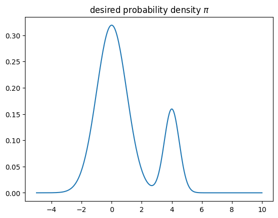
To see where the difficulties in estimating the error come from, let us have a look at a rather artificial toy problem in which the state space is \(\mathbb{R}\) and the desired distribution of the random variable \(X\) displays two peaks,
Suppose we wish to estimate the expectation value of the observable \(f(x)=x\), which is \(\mathbb{E}[f(X)] = \mathbb{E}[X] = 4/5\), using a MCMC.
import numpy as np
rng = np.random.default_rng()
import matplotlib.pylab as plt
%matplotlib inline

def gaussian(mu,sigma,x):
    return np.exp(-(x-mu)*(x-mu)/(2*sigma*sigma))/(sigma*np.sqrt(2*np.pi))

def distribution_pi(x):
    return 0.8*gaussian(0,1,x) + 0.2*gaussian(4,0.5,x)

xrange = np.linspace(-5,10,300)
plt.plot(xrange,distribution_pi(xrange))
plt.title(r"desired probability density $\pi$")
plt.show()
To design a Markov chain \(X_0,X_1,\ldots\) with the desired stationary distribution, we apply the Metropolis-Hastings acceptance to the proposal \(X_i + U\) for the next state \(X_{i+1}\), where \(U\) is a uniform random variable in \((-\delta,\delta)\) with \(\delta = 0.7\). Since \(U\) has a symmetric distribution, the proposal density \(q(x,y)\) is symmetric as well, and therefore the appropriate acceptance probability is \(A(x\to y) = \min(1,\pi(y)/\pi(x))\) with \(x=X_i\) and \(y=X_i+U\). As initial state we choose a rather atypical value \(X_0 = -20\). The following code samples the first 15000 steps of the Markov chain and displays plots of \(X_n\) (sometimes called traces) for three different ranges of the time \(n\), together with the estimates of \(\mathbb{E}[f(X)]\) stemming from the time average in the corresponding range.
def MH_step(current,delta,pi):
    proposal = current + rng.uniform(-delta,delta)
    return proposal if rng.uniform() < pi(proposal)/pi(current) else current

def sample_chain(start,delta,pi,n):
    chain = np.zeros(n+1)
    chain[0] = start
    for i in range(n):
        chain[i+1] = MH_step(chain[i],delta,pi)
    return chain

delta = 0.7
start_x0 = -20
chain = sample_chain(start_x0,delta,distribution_pi,15000)
ranges = [range(1,201),range(201,801),range(801,15001)]
fig, ax = plt.subplots(1,len(ranges),figsize=(16,4))
for i in range(len(ranges)):
    ax[i].plot(ranges[i],chain[ranges[i]])
    ax[i].set_ylim(-22 if i==0 else -8,8)
    time_average = np.mean(chain[ranges[i]])
    title = "time average (i = {}...{}) = {:.3f}".format(ranges[i][0],ranges[i][-1],time_average)
    ax[i].title.set_text(title)
    ax[i].set_xlabel("i")
    ax[i].set_ylabel("$X_i$")
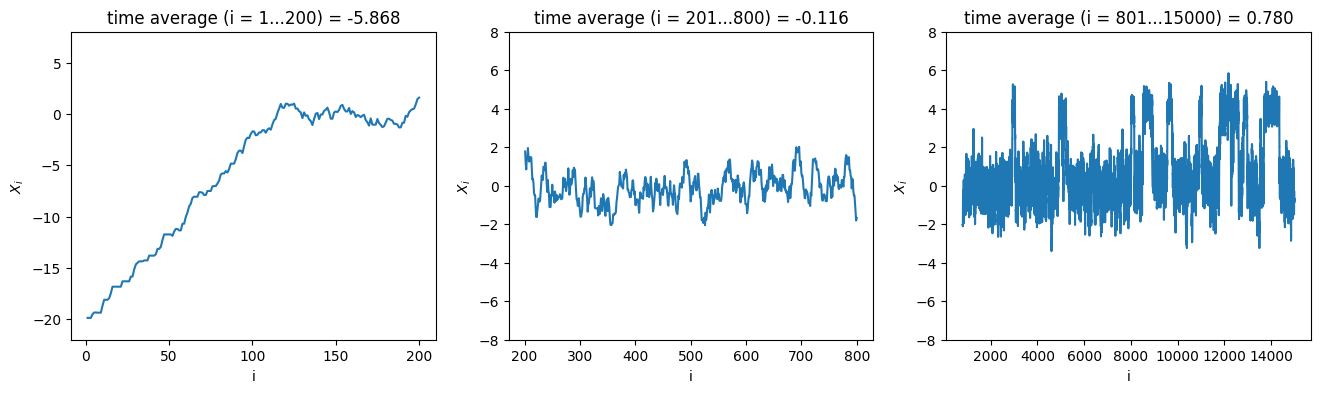
The first two estimates are (most likely) not particularly close to the exact value \(\mathbb{E}[X]=0.8\), but for two different reasons.
5.1.1. Equilibration#
It is clear that the time average \(\frac{1}{n} \sum_{i=1}^n X_i\) for \(n=200\) is very much biased by the atypical starting point \(X_0 = -20\). This may seem artificial, since we chose deliberately to start in an atypical point, but in most applications of MCMC the situation is as bad or worse: any starting point \(X_0\) we are able construct by hand in a high-dimensional sample space is almost guaranteed to be very atypical, in the sense that there are observables \(f : \Gamma \to \mathbb{R}\) such that \(f(X_0)\) is many sigmas away from \(\mathbb{E}[f(X)]\). What we are seeing is that the probability density \(f_{X_i}(x)\) for \(i \leq 200\), is not yet close to the desired distribution \(\pi(x)\). The time \(\tau_{\mathrm{eq}}\) it takes to approach \(\pi(x)\) is called the equilibration time, which appears to be at least \(\tau_{\mathrm{eq}}\geq 200\) in this case. Of course, the contribution of the first \(200\) terms to the time average \(\frac{1}{n}\sum_{i=1}^n f(X_i)\) will become negligible when \(n\to\infty\), but can very much affect the estimate when \(n\) is limited, because the atypical configurations \(X_i\) may contribute excessive values \(f(X_i)\) to the sum.
A common practice is therefore to discard the first \(b\) configurations in the time average, where \(b\) is chosen to ensure \(b\geq \tau_{\mathrm{eq}}\) to the best of our knowledge. This means that we take
as our best estimate of the \(\mathbb{E}[f(X)]\). The first \(b\) steps in a MCMC simulation, in which we discard the observable \(f(X_i)\) (and sometimes not measure \(f(X_i)\) at all), is often called the equilibration, thermalization, or burn-in phase of the simulation. In effect, what equilibration exploits is that, although the limit of the time average is independent of the distribution of \(X_0\), the convergence will be faster if the distribution of \(X_0\) is closer to \(\pi\). This is achieved by taking the random state \(X_b\) as a new effective starting point \(X_0\) of the chain (which by the convergence theorem is close to \(\pi\) for \(b\) large). We will see a technique to gauge \(\tau_{\mathrm{eq}}\) below in the case of the Ising model.
5.1.2. Autocorrelation#
Suppose we know for our example that at time \(i\geq b=200\) the distribution of \(X_i\) is already sufficiently close to \(\pi(x)\). Why is our estimate based on the time average \(i=201,\ldots,800\) still not great, even though we have a decent 600 data points? The reason should be intuitively clear: the states \(X_i\) are far from independent, meaning that each new state only gives us a tiny bit of extra information on the distribution \(\pi\). There is dependence in a trivial sense because our Markov chain is setup such that \(|X_{i+1} - X_i| < \delta\), so the chain cannot wander far in a few steps. More serious is that the distribution \(\pi\) has two peaks, in the vicinity of which the Markov chain likes to stay, separated by a barrier where \(\pi(x)\) is very small. This means that it takes a sequence of probabilistically unlikely steps for the chain to transition between the two regions, so it happens only rarely. The dependence in this example therefore persists over a large number of steps, e.g. you can imagine from looking at the plot that when \(X_i\) is in the vicinity of the first peak the probability that \(X_{i+200}\) is also in this vicinity is larger than if \(X_i\) was in the vicinity of the second peak, i.e. \(\mathbb{P}(X_{i+200} \in (3,5) | X_{i} = 4)\) is significantly larger than \(\mathbb{P}(X_{i+200} \in (3,5) | X_{i} = 0)\). For a good approximation of the desired distribution \(\pi\) we need many transitions between the two regions to have occurred, showing the necessity of performing many steps in the Markov chain (the last plot shows \(\pm 20\) transitions in the first 15000 steps).
Let us try to get a quantitative grasp on the error. To this end we assume that \(\operatorname{Var}(f(X)) < \infty\) and that \(X_0\) has exactly the stationary distribution \(\pi(x)\) (perhaps obtained by performing equilibration for a long time \(b\) and then resetting the label \(i\) of the state \(X_i\) to \(0\)). By construction of the stationary distribution, the same holds for all \(X_i\) with \(i\geq 0\). In this case \(\overline{f(X)}_n=\frac{1}{n}\sum_{i=1}^n f(X_i)\) is an unbiased estimator for \(\mathbb{E}[f(X)]\) since
For the variance we have
where \(\rho(t)\) is the autocorrelation
We can estimate the latter via the sample autocovariance,
from which one obtains the sample autocorrelation as
by normalizing \(\bar{\gamma}(t)\) by the sample variance \(\bar{\gamma}(0)\). For completeness we should mention that variations of the formula (5.2) are used in the literature, for instance one in which the factor \(1/(n-t)\) is replaced by \(1/n\). In each case the result agrees in the limit of large \(n\) when \(t\) is kept fixed, and differences only become noticeable when \(t\) is of the same order as \(n\). The formula (5.2) is sometimes called the unbiased sample autocorrelation, but this is a bit of a misnomer because it is only unbiased if we replace \(\overline{f(X)}_n\) by the known mean \(\mathbb{E}[f(X)]\). The formula with \(1/n\) is often found to be more stable numerically when \(t\) approaches \(n\), so keep that in mind.
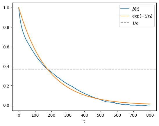
One may be tempted to take the sample autocorrelation \(\bar{\rho}(t)\) and plug it in (5.1), to get an error estimate. However, in practice this rarely works, because the statistical errors in \(\bar{\rho}(t)\) grow large when \(t\) becomes of the order of \(n\). It is often more convenient to estimate an autocorrelation time \(\tau_f\) under the assumption that \(\bar{\rho}(t)\) decays exponentially, i.e. \(\bar{\rho}(t)\approx e^{-t/\tau_f}\). This can be done either by fitting an exponential curve or, slightly less accurately, by taking \(\tau_f\) to be the first time \(t\) that \(\bar{\rho}(t)\) drops below \(1/e\),
If \(1 \ll \tau_f \ll n\), then
Therefore a rough \(1\sigma\)-estimate becomes
Intuitively, we can understand this result in comparison with the i.i.d.-case, where the \(2\tau_f\) factor was missing from the square root. Averaging over \(f(X_i)\) over all times \(i=1,2,\ldots,n\) is essentially as good as averaging \(f(X_i)\) at times \(i=0,2\tau_f,4\tau_f,\ldots\). In the latter case the samples are almost independent, but we have only \(n/(2\tau_f)\) of them. The values that were skipped were sufficiently correlated that they did not contribute much to the accuracy of the average. Therefore the error is as if we were looking at a sequence of \(n/(2\tau_f)\) i.i.d. samples.
def sample_autocovariance(x,tmax):
    '''Compute the sample autocorrelation of the time series x
    for t = 0,1,...,tmax-1.'''
    x_shifted = x - np.mean(x)
    return np.array([np.dot(x_shifted[:len(x)-t],x_shifted[t:])/(len(x)-t)
                     for t in range(tmax)])

def find_correlation_time(autocov):
    '''Return the index of the first entry that is smaller than autocov[0]/e or the length of autocov if none are smaller.'''
    smaller = np.where(autocov < np.exp(-1)*autocov[0])[0]
    return smaller[0] if len(smaller) > 0 else len(autocov)

tmax = 800
burnin = 1000
chain = sample_chain(0,delta,distribution_pi,100000)[burnin:]
autocov = sample_autocovariance(chain,tmax)
autocorr_time = find_correlation_time(autocov)
print("autocorrelation time =",autocorr_time)
error = np.sqrt(2*autocorr_time*autocov[0]/len(chain))
print("E[X] = {:.3f} +- {:.3f}".format(np.mean(chain),error))

plt.plot(autocov/autocov[0])
plt.plot(np.exp(-np.arange(tmax)/autocorr_time))
plt.axhline(np.exp(-1),linestyle='--',color='0.5')
plt.xlabel("t")
plt.legend([r"$\bar{\rho}(t)$",r"$\exp(-t / \tau_f)$",r"$1/e$"])
plt.show()
autocorrelation time = 175
E[X] = 0.798 +- 0.110
By running the above code several times, you will notice that the error is in the right ballpark, but is perhaps not as accurate and stable as you would like. In order to arrive at the error we had to make several assumptions and approximations that necessarily introduce systematic biases in the error estimate. Most notably \(\hat{\rho}(t)\) is not necessarily well-approximated by an exponential decay \(e^{-t/\tau_f}\), even in the limit of large \(n\). We will see more robust and versatile error analysis methods later. Nevertheless, it is almost always a good idea when attacking a problem with MCMC to quickly get an order-of-magnitude estimate of the correlation time \(\tau_f\) of the observable \(f:\Gamma \to \mathbb{R}\) of interest, for two reasons:
You get an order-of-magnitude estimate of the number \(n\) of Markov chain steps needed to reach a desired accuracy.
If measuring the observable \(f(X_i)\) on a given configuration \(X_i\) is computationally expensive, you could choose to perform the measurement only once every \(\tau_f\) steps (or at least that order of magnitude) without increasing the error much. This is called thinning (see below).
5.2. MCMC simulation of the 2D Ising model#
Let us return to the more interesting ferromagnetic Ising model on a 2D lattice of size \(w\times w=N\). We have seen last week how to design a Markov chain on \(\Gamma = \{-1,1\}^N\) that approaches the desired Boltzmann distribution
Since \(J\) and \(\beta = 1/(k_{\mathrm{B}}T)\) only appear in the combination \(J\beta\) and we will only consider the ferromagnetic case \(J>0\), we will set \(J=1\) in the following for convenience. At each step of the Markov chain a uniform random site \(i\) is selected and a flip \(s_i \to s_i'=-s_i\) is proposed. We derived that the appropriate Metropolis-Hastings acceptance probability of this move \(s\to s'\) is
A natural observable is the magnetization \(M(s) = \sum_{i=1}^N s_i\) and its normalized version, the magnetization per spin \(m(s) = M(s)/N\). However, it is easy to see that \(\mathbb{E}[M(s)] = 0\) due to the symmetry of the two spin states \(\pm 1\):
So it is better to consider the absolute magnetization \(|M(s)|\). We can easily figure out the behaviour in the low- and high-temperature limit. In the limit \(\beta \to \infty\) (or \(T\to 0\)) the only two states with positive probability \(\pi(x)\) are the two completely aligned states, hence \(\mathbb{E}[|m(s)|] = 1\). When \(\beta = 0\) (or \(T\to\infty\)) the distribution \(\pi(x)\) is uniform on all spin states. The difference between the number of \(+1\) and \(-1\) spins is then of the order \(\sqrt{N}\), so \(\mathbb{E}[|m(s)|] \approx N^{-1/2}\) is very small for decent size lattices. Another natural observable is the energy \(H(s)\) itself, which, up to normalization and constant shift, counts the number of aligned nearest neighbor pairs in the configuration \(s\).
Our goal will be to estimate the mean (absolute) magnetization \(\mathbb{E}[|M(s)|]\) and mean energy \(\mathbb{E}[H(s)]\) for a range of different temperatures. Preferably we would like to vary the lattice size as well, but for now we will concentrate on a fixed size \(N = 16\times 16=256\).
5.2.1. Equilibration#
As we have seen in the toy problem above, it is important as a first step to get a rough idea of the equilibration time. It is customary to measure equilibration times (and other times in the simulation) not in units of individual Markov chain transitions, but in sweeps:
So let us have a look at the traces of \(M(s)\) and \(H(s)\) for three different initial configurations: the uniformly random configuration; a completely aligned configuration; and the completely anti-aligned configuration.
def attempt_spin_flip_for_trace(config,boltzmannfactor):
    '''Perform Metropolis-Hastings transition on config and return
    change in magnetization and energy.'''
    w = len(config)
    i,j = rng.integers(0,w,2)
    neighbour_sum = config[i,j] * (config[(i+1)%w,j] + config[(i-1)%w,j] +
                                   config[i,(j+1)%w] + config[i,(j-1)%w])
    if neighbour_sum <= 0 or rng.random() < boltzmannfactor**neighbour_sum:
        config[i,j] = -config[i,j]
        return 2*config[i,j], 2*neighbour_sum
    else:
        return 0, 0

def compute_energy(config):
    '''Compute the energy H(s) of the state config (with J=1).'''
    h = 0
    w = len(config)
    for i in range(w):
        for j in range(w):
            h -= config[i,j] * (config[i,(j+1)%w] + config[(i+1)%w,j])
    return h

def compute_magnetization(config):
    '''Compute the magnetization M(s) of the state config.'''
    return np.sum(config)

def get_MCMC_trace(config,beta,n):
    '''Sample first n steps of the Markov chain and produce trace
    of magnetization and energy.'''
    boltz = np.exp(-2*beta)
    trace = np.zeros((n,2))
    # set the initial magnetization and energy ...
    m = compute_magnetization(config)
    h = compute_energy(config)
    for i in range(n):
        dm, dh = attempt_spin_flip_for_trace(config,boltz)
        # ... and update them after each transition
        m += dm
        h += dh
        trace[i][0] = m
        trace[i][1] = h
    return trace

def uniform_init_config(width):
    '''Produce a uniform random configuration.'''
    return 2*rng.integers(2,size=(width,width))-1

def aligned_init_config(width):
    '''Produce an all +1 configuration.'''
    return np.ones((width,width),dtype=int)

def antialigned_init_config(width):
    '''Produce a checkerboard configuration'''
    if width % 2 == 0:
        return np.tile([[1,-1],[-1,1]],(width//2,width//2))
    else:
        return np.tile([[1,-1],[-1,1]],((width+1)//2,(width+1)//2))[:width,:width]

def plot_ising(config,ax,title):
    '''Plot the Ising configuration.'''
    ax.matshow(config, vmin=-1, vmax=1, cmap=plt.cm.binary)
    ax.title.set_text(title)
    ax.set_yticklabels([])
    ax.set_xticklabels([])
    ax.set_yticks([])
    ax.set_xticks([])

# set parameters
beta = 0.33
width = 16
sweeps = 200
nsites = width * width
length = sweeps * nsites
initializers = [uniform_init_config, aligned_init_config, antialigned_init_config]
labels = ["uniform","aligned","anti-aligned"]

# produce the traces and plot initial and final configurations
traces = []
fig, ax = plt.subplots(2,3,figsize=(8,4))
for i, init in enumerate(initializers):
    config = init(width)
    plot_ising(config,ax[0][i],labels[i] + " (initial)")
    traces.append(get_MCMC_trace(config,beta,length))
    plot_ising(config,ax[1][i],labels[i] + " (final)")
plt.show()

# plot magnetization traces
fig, (ax1,ax2) = plt.subplots(1,2,figsize=(15,4))
xrange = np.arange(length)/nsites
for i in range(3):
    ax1.plot(xrange,np.abs(traces[i][:,0]/nsites))
ax1.legend(labels)
ax1.set_xlabel("sweeps")
ax1.set_ylabel("|m|")
ax1.title.set_text("trace of magnetization per spin")

# plot energy traces
for i in range(3):
    ax2.plot(xrange,traces[i][:,1]/(2*nsites))
ax2.legend(labels)
ax2.set_xlabel("sweeps")
ax2.set_ylabel("H/2N")
ax2.set_ylim(-1,0)
ax2.title.set_text("trace of energy per edge")
plt.show()
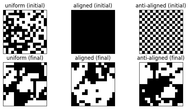
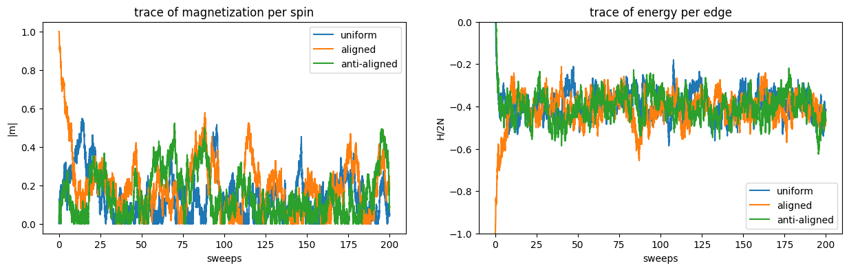
In equilibrium, i.e. when the Markov chain has approached the stationary distribution, the three curves should be close together, or at least fluctuating within the same interval. The equilibration time \(\tau_{\mathrm{eq}}\) is therefore at least as large as the time it takes for the traces to meet each other. Judging from the plot \(\tau_{\mathrm{eq}} \gtrsim 25\text{ sweeps}\). Note also that the magnetization appears to take longer to reach equilibrium. This is a general phenomenon: in principle we should look at a large collection of observables and wait until all traces have suitable converged to conclude on the equilibration time. In practice, however, if it is the magnetization \(|m|\) we wish to estimate, it is typically regarded to be sufficient that its own trace displays equilibrium. To be safe, it is a good idea to spend a number of sweeps in the equilibration phase that is a multiple of the suspected equilibration time \(\tau_{\mathrm{eq}}\). In this case we choose to equilibrate with 500 sweeps.
5.2.2. Autocorrelation#
Next we need an order of magnitude estimate of the autocorrelation time.
# gather the required trace
equil_sweeps = 500
autocorr_sweeps = 1600
length = nsites * (equil_sweeps + autocorr_sweeps)
config = uniform_init_config(width)
trace = get_MCMC_trace(config,beta,length)[nsites * equil_sweeps:]

# compute the autocorrelation over a time difference of 60 sweeps
tmax = nsites * 60
fig, ax = plt.subplots(1,2,figsize=(15,4))
for i in range(2):
    autocov = sample_autocovariance(trace[:,i],tmax)
    autocorr_time = find_correlation_time(autocov)
    ax[i].plot(np.arange(tmax)/nsites,autocov/autocov[0])
    ax[i].plot(np.arange(tmax)/nsites,np.exp(-np.arange(tmax)/autocorr_time))
    ax[i].axhline(np.exp(-1),linestyle='--',color='0.5')
    ax[i].set_xlabel("t")
    ax[i].title.set_text("{} autocorrelation time = {:.1f} sweeps"
                         .format(["magnetization","energy"][i],autocorr_time/nsites))
    ax[i].legend([r"$\bar{\rho}(t)$",r"$\exp(-t / \tau_{f})$",r"$1/e$"])
plt.show()
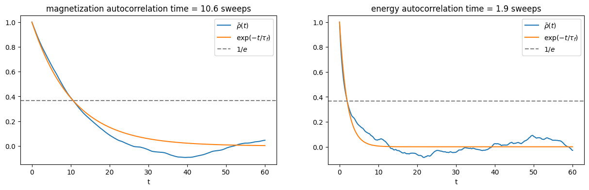
Here we see a similar phenomenon that the estimated autocorrelation time depends on the observable at hand.
5.2.3. Thinning#
We see that for this particular temperature the autocorrelation time is of the order of several sweeps. We could go ahead to estimate the mean magnetization from the trace and calculate the error from the sample variance and autocorrelation time. Instead, let us use the estimate to perform thinning: we re-run the simulation with a larger number of sweeps, but this time we only perform a measurement every \(m\) sweeps. We choose \(m\) between \(1\) and \(\tau_{|M|}\), say \(m=4\). Why? Taking \(m \gtrsim \tau_{|M|}\) would be wasteful, because the magnetization values are already largely uncorrelated after such a time interval. An advantage of thinning is that we do not need to keep track of the observables at every Markov step, saving computation time. However, this means that we have to compute the magnetization and energy every time we wish to measure it, which requires visiting all \(N\) sites. This will take about the same order of time as performing \(N\) transitions, i.e. \(1\) sweep. A good rule of thumb is to spend less than half of the simulation time on measurements, implying that we should take \(m \gtrsim 1\). Let’s gather some data with the choice \(m=4\).
def attempt_spin_flip(config,boltzmannfactor):
    '''Perform Metropolis-Hastings transition on config.'''
    w = len(config)
    i,j = rng.integers(0,w,2)
    neighbour_sum = config[i,j] * (config[(i+1)%w,j] + config[(i-1)%w,j] +
                                   config[i,(j+1)%w] + config[i,(j-1)%w])
    if neighbour_sum <= 0 or rng.random() < boltzmannfactor**neighbour_sum:
        config[i,j] = -config[i,j]

def run_ising_MCMC(config,beta,n):
    '''Perform n steps of the MH Markov chain on config.'''
    boltz = np.exp(-2*beta)
    for _ in range(n):
        attempt_spin_flip(config,boltz)

equil_sweeps = 500
measure_sweeps = 4
num_measurements = 600

# equilibration phase
config = uniform_init_config(width)
run_ising_MCMC(config,beta,equil_sweeps * nsites)

# measurement phase
magnetizations = np.zeros(num_measurements)
energies = np.zeros(num_measurements)
for i in range(num_measurements):
    run_ising_MCMC(config,beta,measure_sweeps * nsites)
    magnetizations[i] = compute_magnetization(config)
    energies[i] = compute_energy(config)

print("estimated mean magnetization per site =", np.mean(np.abs(magnetizations))/nsites)
print("estimated mean energy per edge =", np.mean(energies)/(2*nsites))
estimated mean magnetization per site = 0.17046875
estimated mean energy per edge = -0.398671875
Suppose we do not quite trust our estimate of the autocorrelation time or we wish to estimate a quantity that is not directly an expectation value but can be computed from the samples, like the magnetic susceptibility
then how can we estimate the error? If we had enough computing resources and patience we would repeat the whole experiment \(k\approx 20\) times independently, compute the desired quantity \(k\) times, and determine the mean and standard error for the resulting i.i.d. random outcomes. Sometimes this is a good way to go, for instance when the equilibration time is very short. Quite often though one would like to base estimates on a single long run of the MCMC. Luckily there are several statistical tricks available that allows us to use a single batch of data multiple times in order to mimic the repetition of a whole experiment, including batching and jackknife resampling.
5.2.4. Batching#
Batching or blocking is a very simple technique to mimic \(k\) repetitions of the experiment, simply by chopping the data set into \(k\) equal size batches, usually between \(10\) and \(1000\). The desired quantity is computed for each batch independently and the outcomes are treated as i.i.d. random variables, for which we know how to estimate the mean and standard error. This procedure is justified when the batch size \(n/k\) is much larger than the autocorrelation time \(\tau_f\), because then most of the measurements in one batch are uncorrelated with those in another batch.
def batch_estimate(data,observable,k):
    '''Devide data into k batches and apply the function observable to each.
    Returns the mean and standard error.'''
    batches = np.reshape(data,(k,-1))
    values = np.apply_along_axis(observable, 1, batches)
    return np.mean(values), np.std(values)/np.sqrt(k-1)

num_batches = 50
magnet_est = batch_estimate(np.abs(magnetizations)/nsites,lambda x: np.mean(x), num_batches)
suscep_est = batch_estimate(magnetizations/nsites,lambda x: beta*nsites*np.var(x), num_batches)
print("mean magnetization: E[|m|] = {:.4f} +- {:.4f}".format(*magnet_est))
print("magnetic susceptibility: chi = {:.4f} +- {:.4f}".format(*suscep_est))
mean magnetization: E[|m|] = 0.1705 +- 0.0076
magnetic susceptibility: chi = 2.4793 +- 0.2001
5.2.5. Jackknife#
Batching works well for estimating expectation values, but can become inaccurate for more elaborate quantities, because individual batches may be too small to sample the quantity well. In such a case an option is to use jackknife resampling. The general idea is simple. Suppose we have divided our data into \(k\) batches. Instead of computing our quantity of interest independently in the \(k\) small batches, we compute in the \(k\) datasets that are obtained by considering \(k-1\) of the \(k\) batches combined, each time leaving one batch out. Of course the \(k\) different values obtained in this way are highly correlated, but one can show that this effect can be compensated by taking the error to be \(\sqrt{k-1}\) times the standard deviation of the \(k\) values (instead of the standard error which is \(1/\sqrt{k-1}\) times the standard deviation).
def jackknife_batch_estimate(data,observable,k):
    '''Devide data into k batches and apply the function observable to each
    collection of all but one batches. Returns the mean and corrected
    standard error.'''
    batches = np.reshape(data,(k,-1))
    values = [observable(np.delete(batches,i,0).flatten()) for i in range(k)]
    return np.mean(values), np.sqrt(k-1)*np.std(values)

num_batches = 50
magnet_est = jackknife_batch_estimate(np.abs(magnetizations)/nsites,
                                      lambda x: np.mean(x), num_batches)
suscep_est = jackknife_batch_estimate(magnetizations/nsites,
                                      lambda x: beta*nsites*np.var(x), num_batches)
print("mean magnetization: E[|m|] = {:.4f} +- {:.4f}".format(*magnet_est))
print("magnetic susceptibility: chi = {:.4f} +- {:.4f}".format(*suscep_est))
mean magnetization: E[|m|] = 0.1705 +- 0.0076
magnetic susceptibility: chi = 3.7212 +- 0.3282
Note that the estimate and error in the case of the expectation value are unchanged compared to the batching method (with the same number of batches), but for quantities that are not expectation values, like the magnetic susceptibility, the result will differ.
5.3. Further reading#
Toy problem is adapted from: Section 11.5 of [Owe13].
Ising model simulation in practice: Chapter 4 of [NB99]. (See in particular Section 3.4 about the error analysis)
An accessible discussion on the different error estimates can be found in [Rum].