A series of lectures given on 21-22 June 2017 at Making Quantum Gravity Computable, Perimeter Institute, Canada.
| Slides | Video recording | |
|---|---|---|
| Part I: Random geometry in 2D | mcdt-part1.pdf | pirsa.org/17060075, pirsa.org/17060076. |
| Part II: Higher dimensions | mcdt-part2.pdf | pirsa.org/17060082, pirsa.org/17060083. |
| Tutorial sessions | Description of the models | pirsa.org/17060079, pirsa.org/17060086. |
The goal of the tutorial sessions is to gain some experience in: handling random two-dimensional geometries, performing measurements, and extracting critical exponents from data analysis.
To this end I provide a computer program randgeom that produces random planar maps on demand subject to several parameters.
randgeomThe simplest way to get the program running is to download one of the precompiled executables. Simply right-click the link next to your operating system and select Save as... You may need to set execution permissions (chmod u=rxw randgeom on Linux/OSX).
| OS | Executable | MD5 checksum |
|---|---|---|
| Linux | randgeom | eb2200d159f5b57be28862c1ece1b56d |
| OSX | randgeom | 53149d6b8b96afe23d121d129039d48e |
| Windows (32bit) | randgeom.exe | 71ed82188a7f8a78d6b802e2d49a7441 |
Alternatively you may compile the c++ source yourself (tested with GNU c++ compiler only). Download source.tar.gz or source.zip and extract all files. Then run the following command (or similar) in the directory to which the files were extracted.
g++ main.cpp -I. -O2 -o randgeomrandgeomrandgeom takes three parameters:
-t followed by A, B, C, or D: the requested model type. -s followed by positive integer S: the requested size S of the planar map measured by number of faces. -n followed by positive integer N: the number N of independent configurations to be returned. The following returns a single random planar map sampled from model A with 4 faces.
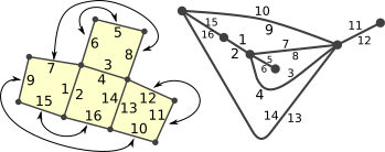
$ ./randgeom -tA -s4 -n1
{{{7,15,2},{16,4,1},{8,6,4},{2,14,3},{6,8,6},{3,5,5},{9,1,8},{5,3,7},{15,7,10},{11,13,9},{12,10,12},
{13,11,11},{10,12,14},{4,16,13},{1,9,16},{14,2,15}}}
The output is formatted as a Mathematica-style nested list of length N, one entry per configuration. Each configuration corresponds to a list of triples of integers describing a planar map through permutations: the
i'th triple corresponds to {n(i),n-1(i),a(i)}, where n and a are the ``next'' and ``adjacent'' permutations (see lecture slides).
The output above corresponds to the following quadrangulation displayed both as a gluing prescription and as a planar map.
In case you prefer to read the output from a different program than Mathematica, you may prefer to receive the data as a space-separated list. To this end one may use the option --spaceseparated:
$ ./randgeom -tA -s2 -n2 --spaceseparated
2
8
3 7 2
8 4 1
5 1 4
2 6 3
7 3 6
4 8 5
1 5 8
6 2 7
8
5 8 2
6 4 1
4 6 4
2 3 3
7 1 6
3 2 5
8 5 8
1 7 7
The output is structured as follows: the first line contains the number N of configurations. Then for each configuration a line with the number H of half-edges, followed by H lines with triples of integers corresponding to
n(i), n-1(i) and a(i) respectively.
randgeom with MathematicaI have prepared an example notebook to read the output of randgeom to perform various manipulations. It also contains pointers on how to measure the three types of observables we discussed in the lecture.
example-analysis.nb
example-analysis.txt (in case your (older) Mathematica has trouble reading the notebook)
randgeom from a c++ program
For those who wish to use c++ to perform measurements, I have prepared a minimal working example to execute randgeom and read output data (tested on Linux only): example-import.cpp.